Quantum Monte Carlo for Aerospace Uncertainty Quantification

High-fidelity aerospace simulations are central to design and mission-critical decision-making. These simulations often involve solving complex partial differential equations (PDEs) with uncertain inputs. While Direct Numerical Simulation (DNS) and Large Eddy Simulation (LES) provide detailed representations of turbulence, their computational demands limit them to academic use cases. As a result, Reynolds-Averaged Navier Stokes (RANS) models remain the primary choice for engineering practice, though they introduce modeling uncertainties.

Uncertainty Quantification (UQ) is essential in this context, as approximations in turbulence models can significantly affect predictions. These uncertainties are broadly classified as aleatory and epistemic. Aleatory uncertainties arise from inherent variability in inputs, such as material properties or boundary conditions, while epistemic uncertainties stem from model inadequacy. Classical Monte Carlo (MC) methods are widely used for UQ but become computationally infeasible for large-scale problems. This limitation motivates the exploration of Quantum Monte Carlo (QMC) methods.

Uncertainty Sources in Aerospace Simulations

Aleatory uncertainties are stochastic and irreducible, often modeled by probability distributions. They propagate through simulations and affect the outputs, such as lift or drag predictions. Epistemic uncertainties, in contrast, are reducible but persist due to turbulence model limitations. Both can be represented in a Bayesian framework, provided sufficient priors exist.

Traditional MC methods require a large number of samples to reduce error, with computational cost scaling as O(1/ε^2) for error ε. This creates bottlenecks when applied to aerospace workflows. Quantum algorithms, which are inherently probabilistic, offer a quadratic improvement in sample complexity via Quantum Amplitude Estimation (QAE).

_{BQP’s approach to uncertainty quantification -}

‍Problem Setup

To evaluate the performance of Quantum Computing-based Monte Carlo (QCMC), a stochastic transient heat conduction problem was considered where the domain was a unit square with uncertainties in thermal conductivity k and the left boundary temperature Tx=0.

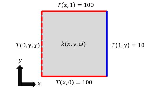
The governing PDE is: cpTt=k.x,y,wT, Tt=0=T0x,y, where ρ is density, c_p is specific heat capacity, and k(x,y,ω) is modeled as a spatially varying random field. The initial condition is a known profile T₀(x,y), while Dirichlet conditions are applied to all edges. The left boundary condition incorporates epistemic uncertainty through a sinusoidal perturbation about the mean temperature.

Representing Sources of Uncertainty

Thermal Conductivity Field: The thermal conductivity is expanded using a truncated Karhunen–Loève (KL) expansion: 

‍

where φn are orthonormal eigenfunctions, λn eigenvalues, and ξn(ω) ~ N(0,1). This approach converts infinite-dimensional randomness into a finite set of uncorrelated random variables.

Boundary Temperature Perturbation: The left boundary temperature condition is defined with a sinusoidal fluctuation: 

Tleft0,y,=Tmean+Tperturbation*sin⁡yLy

where χ is a Gaussian random variable that introduces variability in frequency. This formulation captures epistemic uncertainty in boundary conditions.

Numerical Discretization

The PDE is solved using explicit finite difference methods on a structured Cartesian grid. Let α = k/ρ c_p denote the thermal diffusivity. The temperature update formula at grid point (i,j) from time step n to n+1 is:

Ti,jn+1=Ti,jn+tx2Ti+1,jn−2Ti,jn+Ti−1,jn+ty2Ti+1,jn,−2Ti,jn+Ti−1,jn.

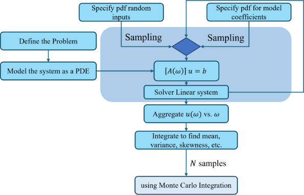
Hybrid Quantum Monte Carlo Workflow

The hybrid QMC approach proceeds in four steps:

1. Model uncertain parameters (flow conditions, geometry tolerances).

2. Encode the UQ problem into quantum circuits using state preparation and amplitude encoding.

3. Apply Quantum Amplitude Estimation (QAE) to estimate statistical metrics with fewer samples.

4. Post-process results classically to compute mean, variance, and confidence bounds.

This workflow leverages the efficiency of quantum subroutines while retaining classical post-processing for robustness.

‍

Quantum Computing-Based Monte Carlo

QCMC estimates the expectation value of a bounded function f(x) over domain x ∈ {0,1}ⁿ:

Efx=, with 0 ≤ f(x) ≤ 1.

Classical MC requires O(1/ε^2) samples to achieve error ε, whereas QCMC reduces this to O(1/ε) using QAE.

Maximum Likelihood Amplitude Estimation

Circuit diagrams for different Quantum Amplitude Estimation (QAE) approaches used in the BQP’s QCMC

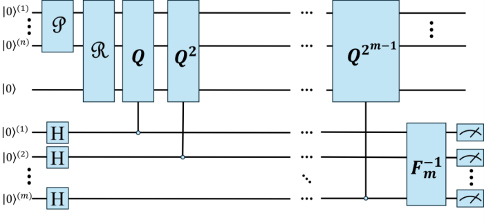
Figure - Quantum Amplitude Estimation (QAE) using the Phase Estimation algorithm

[The circuit includes 𝑚 ancillary qubits and 𝑛 + 1 state qubits. 𝐹−1 𝑚 represents the Inverse Quantum Fourier Transform (QFT), and 𝑄 denotes the Grover operator]

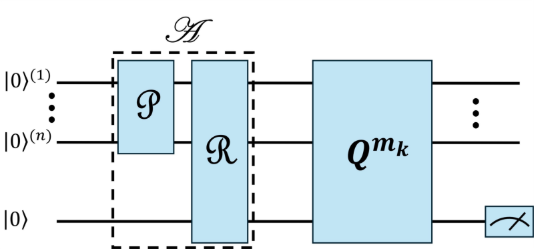
Figure - Quantum Amplitude Estimation (QAE) without the Phase Estimation algorithm

[The circuit has n + 1 state qubits. 𝑄 here is the Grover operator]

Figure - Circuit diagram for Quantum Amplitude Estimation (A(P, 𝑖, 𝛽, 𝑛, 𝜔)) function and probability distribution encoding

[Here, 𝛼 = 𝑛𝜔𝑥𝑙 − 𝛽, and 𝜃 = 𝑛𝜔Δ, where 𝑥𝑙 is the lower limit of the integral and Δ is the spacing between each point in the integral.]

Alternative to Quantum Phase estimation -

Instead of relying on Quantum Phase Estimation, BQP adopts Suzuki’s Maximum Likelihood Amplitude Estimation (MLAE). The method avoids deep circuits and controlled operations, making it practical for near-term quantum devices. For each Grover iteration count mk, the likelihood of observing a 'good' outcome is: 

Lkhk;k=sin2⁡2mk+1ahkcos2⁡2mk+1aNk−hk.

where h_k is the count of good outcomes and N_k the total samples. The joint likelihood is maximized to estimate the amplitude.

Fourier-Based Function Decomposition

Encoding arbitrary functions into quantum circuits can be expensive. To reduce depth, BQP employs a Fourier expansion:

fxa02+ancos⁡nx+bnsin⁡nx.

Expectation values of cosine and sine terms are estimated using QAE circuits:

Cosine components - 

 xcos⁡nx1−2QAEAP,i,0,n,,q

Sine components - 

The final expectation of f(x) is reconstructed as:

Statistical Analysis used for the case study -

At representative domain points such as (0.5, 0.5), probability distribution functions are constructed using Kernel Density Estimation (KDE). Statistical moments are then computed:

‍

Monte Carlo and QCMC are both applied to these calculations. QCMC demonstrates lower sample complexity while retaining statistical accuracy, showing promise for large-scale aerospace UQ tasks.

The integration of QCMC into aerospace workflows provides a structured pathway to address uncertainty quantification challenges. By combining classical discretization methods with quantum-enhanced sampling, the framework achieves improved efficiency in propagating and analyzing uncertainties. The Fourier-based decomposition and MLAE technique further adapt the algorithm for near-term quantum devices.

This hybrid approach underscores how quantum computing can complement existing high-performance computing platforms, enabling more reliable and computationally feasible uncertainty quantification in aerospace design and analysis.