How Do You Optimize Rocket Nozzle Design? Constraints, Methods, and Practical Execution

Rocket nozzle performance depends on constrained, multi-variable optimization.

Design teams balance thermodynamic efficiency, structural integrity, and manufacturability within tight operational envelopes. Every constraint interacts.

• This article covers dominant constraints that limit rocket nozzle design performance
• Three optimization methods are compared, including quantum-inspired approaches using BQP
• Step-by-step execution workflows are provided for each method with failure modes

Execution details for each method follow, specific to nozzle geometry and operating conditions.

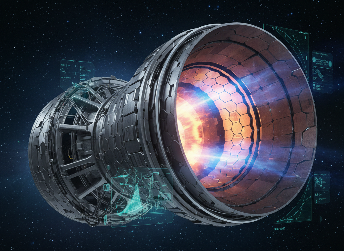
What Limits Rocket Nozzle Performance?

Optimization begins by identifying the dominant constraints specific to the nozzle.

The following limiting factors represent widely recognized engineering constraints in nozzle design.

1. How Does Thermal Load Distribution Constrain Nozzle Design?

Nozzle walls experience extreme thermal gradients during combustion.

Material selection and cooling channel geometry must account for heat flux across the expansion profile.

Thermal limits directly constrain wall thickness, expansion ratio, and coolant flow optimization.

2. How Does Geometric Expansion Ratio Affect Performance?

The ratio of exit area to throat area governs exhaust velocity and thrust efficiency.

It is a primary design variable in nozzle contour optimization.

Altitude-dependent performance tradeoffs restrict the viable range of expansion ratios for any mission profile.

3. How Does Structural Integrity Under Pressure Limit Design Options?

Internal chamber pressures impose significant mechanical stress on nozzle structures.

Material yield limits and fatigue cycles define allowable operating envelopes.

Pressure constraints reduce the feasible design space for optimization solvers.

4. How Do Manufacturing Tolerances Constrain Optimization?

Complex nozzle contours require precision fabrication methods.

Tolerances in additive or subtractive manufacturing affect as-built performance versus design intent.

Tight fabrication limits constrain how aggressively solvers can push geometric optimization boundaries.

Key takeaway: Thermal, geometric, structural, and manufacturing constraints are coupled. Optimizing one variable in isolation risks violating limits in another.

What Are the Optimization Methods for Rocket Nozzles?

Three methods apply to nozzle-level optimization with distinct strengths.

How Does Quantum-Inspired Optimization Using BQP Work for Nozzle Design?

BQPhy applies quantum-inspired evolutionary optimization algorithms to classical HPC infrastructure, targeting large combinatorial design spaces.

• Parallel search across high-dimensional nozzle design variables without gradient dependence
• Reduced convergence cycles for coupled thermal-structural-geometric constraints
• HPC-compatible execution that integrates with existing simulation environments
• High-dimensional constraint handling suited to multi-objective optimization problems

For nozzle optimization, BQPhy enables simultaneous exploration of expansion ratio, wall contour, and cooling geometry without simplifying coupled physics interactions.

Best-fit scenarios for BQP on this component:

• Nozzle contour optimization with more than three coupled constraint categories
• Design exploration where classical solvers hit convergence limits
• Trade studies across mission-variable expansion ratios requiring broad search
• Integration with existing HPC clusters running aerospace optimization techniques

What Are the Step-by-Step Execution Steps for Nozzle Optimization Using BQP?

The following steps reflect a logical workflow consistent with documented BQPhy platform capabilities.

Step 1: Define Nozzle Design Variable Bounds

Establish parameter ranges for throat diameter, expansion ratio, wall contour control points, and cooling channel geometry.

Each variable bound must reflect material and mission constraints.

Step 2: Encode Coupled Constraint Functions

Map thermal, structural, and geometric constraints into the optimization formulation as coupled penalty or feasibility functions.

Constraint encoding determines solver search quality.

Step 3: Configure Quantum-Inspired Search Parameters

Set population size, iteration limits, and convergence thresholds within the Quantum Optimization Solution environment.

Parameters must balance exploration breadth with computational budget.

Step 4: Execute Parallel Design Evaluation

Run the quantum-inspired evolutionary solver across the defined design space using HPC-compatible parallel execution.

Monitor convergence behavior across each design variable.

Step 5: Filter Pareto-Optimal Nozzle Candidates

Extract non-dominated designs from the solution set based on thrust efficiency, thermal margin, and structural safety factor.

Filtering reduces candidates to physically viable configurations.

Step 6: Validate Top Candidates Against CFD Baseline

Run high-fidelity CFD simulations on the top-ranked nozzle geometries to confirm performance predictions.

Validation catches optimizer assumptions that diverge from flow physics.

Step 7: Select Final Geometry for Fabrication Review

Choose the design that satisfies all constraints and aligns with manufacturing feasibility for the target production method.

This step bridges optimization output to production readiness.

What Are the Failure Modes with BQP?

Solver convergence may stall if constraint functions are poorly scaled relative to design variable magnitudes.

Overly broad variable bounds increase computation without improving solution quality for constrained nozzle geometries.

Key takeaway: BQP is suited to coupled, high-dimensional nozzle problems where classical solvers reach convergence limits. Constraint scaling and variable bounding are critical to execution quality.

How Does CFD-Coupled Adjoint Optimization Apply to Nozzle Design?

Adjoint methods compute gradients of objective functions with respect to all design variables in a single adjoint solve.

This method fits nozzle optimization because contour shape directly governs flow separation, shock structure, and thrust loss.

It performs best when refining a baseline nozzle geometry toward a local optimum.

What Are the Execution Steps for CFD-Coupled Adjoint Nozzle Optimization?

The following steps reflect standard adjoint-based design optimization software practice applied to nozzle geometry.

Step 1: Generate Baseline Nozzle Flow Solution

Run a converged CFD simulation on the initial nozzle geometry to establish the primal flow field.

The baseline solution anchors all subsequent gradient computations.

Step 2: Define Thrust-Based Objective Function

Specify the optimization objective as thrust coefficient or specific impulse derived from nozzle exit conditions.

Objective formulation must reflect the mission-critical performance metric.

Step 3: Solve Adjoint Equations for Shape Sensitivity

Compute the adjoint field to obtain gradients of the objective with respect to every surface mesh node.

This step reveals which contour regions most influence performance.

Step 4: Apply Surface Deformation Along Gradient

Deform the nozzle wall contour in the direction of steepest improvement indicated by adjoint sensitivity.

Deformation magnitude must respect mesh quality limits.

Step 5: Re-Solve Flow and Iterate to Convergence

Run the updated geometry through CFD, recompute adjoint sensitivities, and repeat until objective improvement plateaus.

Convergence typically requires multiple flow-adjoint cycles.

Step 6: Verify Structural Feasibility of Optimized Contour

Check the optimized wall profile against thermal and pressure load constraints using structural analysis.

Adjoint methods do not inherently enforce structural limits.

What Are the Failure Modes for Adjoint Optimization?

Adjoint solvers can fail when flow features like shocks move discontinuously between design iterations.

Local optima trapping is inherent. Adjoint methods cannot explore globally across the design space.

Key takeaway: Adjoint optimization excels at refining near-optimal nozzle contours but cannot replace broad design space exploration methods.

How Does Surrogate-Assisted Evolutionary Optimization Work for Nozzles?

Surrogate models approximate expensive CFD evaluations using trained response surfaces built from sampled nozzle designs.

This approach reduces the computational cost of evolutionary search across large nozzle design spaces with complex optimization use cases.

It performs best for early-stage multi-objective trade studies with limited compute budgets.

What Are the Execution Steps for Surrogate-Assisted Nozzle Optimization?

The following steps reflect established engineering optimization software practice.

Step 1: Sample Initial Nozzle Design Points

Generate a space-filling set of nozzle geometries using Latin hypercube or similar sampling across key design variables.

Sample quality determines surrogate model accuracy.

Step 2: Evaluate Samples with High-Fidelity CFD

Run full CFD simulations on each sampled design to produce objective and constraint response data.

This is the most computationally expensive step.

Step 3: Train Surrogate Response Surface

Fit a surrogate model (Kriging, radial basis function, or polynomial) to the sampled CFD results.

Model accuracy must be validated before optimization proceeds.

Step 4: Run Evolutionary Search on Surrogate

Execute a genetic algorithm or evolutionary optimizer using the surrogate as a fast objective evaluator.

Surrogate-based search explores far more candidates than direct CFD evaluation allows.

Step 5: Infill High-Uncertainty Regions

Identify designs where surrogate prediction uncertainty is highest and evaluate them with CFD to improve model fidelity.

Infill sampling prevents the optimizer from exploiting surrogate errors.

Step 6: Extract and Validate Final Nozzle Designs

Select top candidates from the surrogate-assisted search and confirm performance with full CFD validation.

Final validation ensures surrogate predictions hold under high-fidelity analysis.

What Are the Failure Modes for Surrogate-Assisted Optimization?

Surrogate accuracy degrades in regions with sparse sampling or nonlinear response behavior.

High-dimensional nozzle problems require large sample counts, partially offsetting computational savings.

Key takeaway: Surrogate methods suit early-stage exploration under compute constraints. Infill sampling discipline is essential for reliable results.

What Key Metrics Should You Track During Rocket Nozzle Optimization?

Thrust Performance

Thrust performance metrics quantify how effectively the nozzle converts combustion energy into directed exhaust momentum.

• Tracks specific impulse and thrust coefficient across operating conditions
• Reveals efficiency losses from flow separation or contour suboptimality
• Enables direct comparison between optimization candidates

These metrics determine whether the optimized nozzle meets mission propulsion requirements.

Thermal Margin

Thermal margin measures the gap between predicted peak wall temperature and the allowable material limit.

• Identifies hot spots that could cause wall failure
• Validates cooling channel adequacy in regeneratively cooled designs
• Constrains viable contour shapes during optimization

Insufficient thermal margin disqualifies otherwise high-performing geometries.

Structural Safety Factor

Structural safety factor compares material yield strength against maximum mechanical stress from chamber pressure and thermal loading.

• Confirms the nozzle can withstand pressure cycles without failure
• Accounts for fatigue under repeated firing conditions
• Bridges optimization results to certification requirements

These metrics decide whether the design is viable for production and flight.

Frequently Asked Questions About Rocket Nozzle Optimization

What is the biggest constraint in rocket nozzle optimization?

Thermal load distribution typically dominates. Peak wall temperatures interact with material limits, cooling design, and geometric contour simultaneously. This coupling makes thermal management the most complex constraint to satisfy during nozzle optimization using any method, including quantum optimization approaches.

How does quantum-inspired optimization differ from genetic algorithms for nozzle design?

Quantum-inspired methods apply principles like superposition-inspired search to improve exploration efficiency across high-dimensional spaces. Standard genetic algorithms rely on crossover and mutation alone. BQPhy's quantum design optimization approach reduces convergence cycles while maintaining constraint feasibility in coupled nozzle problems.

When should surrogate-assisted optimization be used instead of direct CFD optimization?

Surrogate methods suit early-stage trade studies where hundreds of candidate evaluations are needed but CFD budgets are limited. Direct CFD optimization is preferred when the design space is narrow and gradient information is reliable for contour refinement.

Why do adjoint methods struggle with rocket nozzle flows?

Adjoint solvers assume smooth gradient fields. Nozzle flows with moving shocks or flow separation create discontinuities that degrade gradient accuracy. This makes adjoint methods better suited for refining near-optimal contours rather than exploring broad design spaces with predictive aviation optimization goals.

What advantage does BQP offer over scaling HPC hardware for nozzle optimization?

BQP delivers algorithmic efficiency gains on existing classical HPC infrastructure. Rather than adding compute capacity to run the same solvers longer, BQPhy applies quantum-inspired evolutionary optimization to reduce convergence cycles and improve solution quality within current hardware budgets.